Introduction
“Can you check if this is significant?”
It was a seemingly innocuous question from a dangerous source: a semi data-literate scientist. The kind who believed, deep in his heart, that small p-values were “good” and large p-values were “erroneous”.
On this day, the man in question had come forth with a large, complex multivariate dataset. He’d manually combed the data, visually inspected it, and hand-picked a hypothesis.
“Can you check if this is significant?”
“I can, but I shouldn’t.”
Fishing for Trouble
On the surface, the above appears pretty innocent. Someone has a dataset, looks at it, and conceives a hypothesis.
The problem, of course, is in the looking. Let’s imagine the problem in the context of xkcd’s jelly bean example. The task in question was to see if there was a link between acne and a certain color of jelly bean.
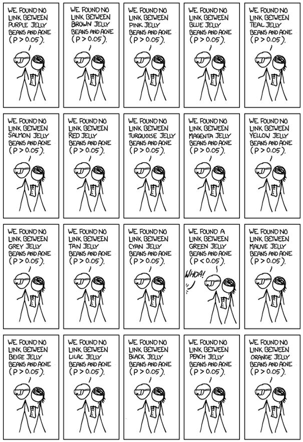
The conclusion, naturally, was absurd.
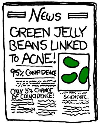
The comic serves as a simple argument for the necessity of multiple corrections. If you run 20 tests at an un-adjusted alpha value of 0.05, you’d expect to reject one on average by random chance in situations where no true relationship exists. As statisticians we’re taught to account for multiple testing with something like a Bonferroni correction or by applying false discovery rate control.
In our example, abiding by the scientist’s request commits the same error from another angle. To bring the two together, imagine that our scientist had, prior to forming a hypothesis, first looked at the jelly-bean data. The scientist rejects many hypotheses via visual inspection (“black jelly beans seem fine”), then comes to the statistician with a proposal.
“Can you check if the link between green jelly beans and acne is significant?”
Applied Example
Let’s consider a (slightly) less abstract example. Suppose we have a drug study, where the concentration of the active compound decreases linearly over time. We might be interested in testing whether the initial concentrations (intercepts) or drug degradation (slope) differ between manufacturing processes (batches).
Below we consider a scenario where a statistician scans datasets, and picks a subset to test for differences in intercept.
A simulation study
In this section, we simulate data and test hypotheses after “looking” at the measurements, to see how this approach alters the properties of our statistical tests. We assume that in each dataset we have two batches and 10 measures for each batch. The real unknown model is for all batches i and for all measures j:
where $\varepsilon_{1,1}, \ldots, \varepsilon_{1, 10}$ and
$\varepsilon_{2,1}, \ldots, \varepsilon_{2, 10}$ are assumed to be independent Gaussian random variables with an expectation equal to $0$ and a variance equal to $0.01$.
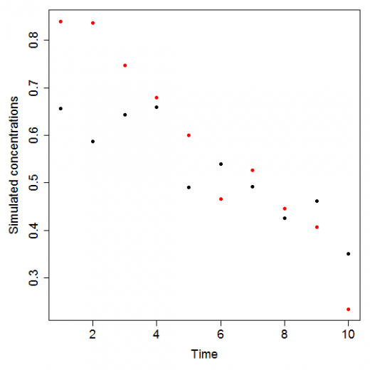
Figure 1: points generated using the above equation for the first batch (black) and the second batch (red).
We moreover choose $t_{i,j}=j$ for all $i \in \{1,2\}$ and all $j \in \{1,\dots,10\}$. That is, both batches are generated from an identical underlying model, with differences in data attributed to random variability. We generate all the $y_{i,j}$’s 10000 times and each time we estimate the parameters of the following model:
A first step to analyse data is often to create a scatterplot. We assume that some statistician will decide to test if the initial concentrations are equal after looking at such scatterplot. To mimic this statistician’s behaviour, we compute for all samples
where $RSS$ is the residual sum of squares. Our statistician will decide to use his test if the value of this indicator is large. To see the link between this indicator and the will to perform this test, we display in Figure 1 the points corresponding to the sample with the largest $\rho$.
For the 1000 samples with the largest values of $\rho$, we then test if $\beta_{1,1} = \beta_{1,2}$. To do so, we use Seber and Lee (2003, Example 4.7, page 107). We choose $\alpha=5\%$. The proportion of statistically significant tests is equal to 47.6%, which is very different from $\alpha$. By contrast, if we perform the test for all samples (instead of just a subset), this proportion becomes 4.83%.
Conclusion
Testing hand-picked hypotheses can be highly misleading, and as shown above, is succeptible to an alarming rate of false positives. For a more formal exploration of this topic, see this blog supplement. Thanks for reading!
References
G. A. F. Seber and A. J. Lee. Linear regression analysis. Wiley Series in Probability and Statistics. John Wiley & Sons, Hoboken, United States of America, 2nd edition, 2003.